POA Ground Reflected

You are here:

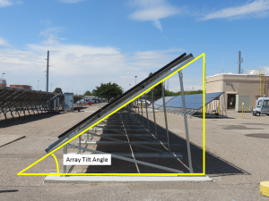
Irradiance on a tilted surface that is reflected off the ground, $E_{g}$ , is calculated as a function of the irradiance on the ground, usually assumed to be $GHI$ , the reflectivity of the ground surface, known as albedo, and the tilt angle of the surface, $\theta_{T,surf}$ :

$E_{g}=GHI\times albedo\times \frac{\left ( 1-\cos \left ( \theta_{T,surf} \right ) \right )}{2}$

The model for ground reflected irradiance $E_{g}$ develops from the following assumptions:

The array is infinitely long.
Irradiance on the ground is uniform and equal to $GHI$ , i.e., horizon blocking and near-field shading by the array is ignored.
Irradiance reflects from the ground equally in all directions, i.e., the ground is a diffuse or Lambertian reflector.
The ground is visible to the array from the point of intersection of the array’s slope projected to the ground, to the infinite horizon.

With these assumptions the model for $E_{g}$ can be derived using a view or configuration factor. The view factor quantifies the fraction of diffuse reflected irradiance from one surface $A_{1}$ that impinges on a second surface $A_{2}$ . In the equation above for $E_g$ , the term $\frac{1-\cos{\theta_{T,surf}}}{2}=F_{A_1 \rightarrow A_2}$ is the view factor from surface $A_1$ , the ground, to surface $A_2$ , the module.

To derive this model, consider an infinite strip $dA_{1}$ on the ground of differential width $dx$ that is parallel to the array. Denote the array’s face as $A_{2}$ , and the view factor from $dA_{1}$ to $A_{2}$ as $F_{dA_{1} \rightarrow A_{2}}$ . The irradiance per unit length (W / m) reflecting from the strip $dA_{1}$ is $GHI \times albedo \times dx$ . The contribution to irradiance per unit length (W / m) on $A_{2}$ from reflected irradiance from $dA_{1}$ is

$dE_{g}=GHI \times albedo \times F_{dA_{1} \rightarrow A_{2}} \times dx$

Let $x$ be a coordinate axis on the ground with origin under the lower, forward edge of the array, parallel to the rear-facing normal vector to the array, with negative direction toward the horizon behind the array. Consider $A_{1}$ to be the half-plane on the ground defined by $x\leq x_{0}$ , and $A_{2}$ to be the rear-facing side of an infinitely long strip of width $L$ above the half plane with edges parallel to the ground. The total irradiance on $A_{2}$ per unit area (W/m2) from irradiance reflected from $A_{1}$ is

$\begin{align*} E_g & = \frac{1}{A_2}\int dE_g = \frac{1}{L_2}\int_{-\infty}^{x_0}GHI\times albedo \times F_{dA_1\rightarrow A_2}dx \\ & = GHI \times albedo \times \int_{-\infty}^{x_0}\frac{F_{dA_1\rightarrow A_2}}{L_2}dx \\ & = GHI \times albedo \times F_{A_1 \rightarrow A_2} \end{align}$

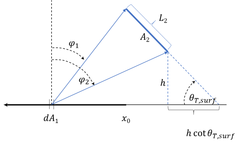
The view factor $F_{dx \rightarrow A_{2}}$ is given by the formula

$F_{dA_{1} \rightarrow A_{2}} = \frac{1}{2} \left( \sin \left( \phi_{2} \right) - \sin \left( \phi_{1} \right) \right)$

( see case B-71 at http://www.thermalradiation.net/tablecon.html)

Rewriting the terms in the equation for $F_{dA_{1} \rightarrow A_{2}}$ as

$\sin \phi_{2} = \cos \left(90 - \phi_{2} \right ) = \frac{x - h \cot \theta_{T,surf}}{\sqrt{\left(x - h \cot \theta_{T,surf} \right )^2 + h^2}}$

$\sin \phi_{1} = \cos \left(90 - \phi_{1} \right ) = \frac{x - h \cot \theta_{T,surf} - L_{2} \cos \theta_{T,surf}}{\sqrt{\left(x - h \cot \theta_{T,surf} - L_{2} \cos \theta_{T,surf} \right )^2 + \left(L_{2} \sin \theta_{T,surf} + h \right )^2}}$

Substituting and evaluating the integral $F_{A_1 \rightarrow A_2} = \int_{-\infty}^{x_0}\frac{F_{dA_1 \rightarrow A_2}}{L_2} dx$ obtains

$F_{A_{1} \rightarrow A_{2}} = \frac{1}{2} \left [L_{2} \cos \theta_{T,surf} - \sqrt{\left( x_{0} - h \cot \theta_{T,surf} \right)^2 + h^2} + \sqrt{ \left( x_{0} - h \cot \theta_{T,surf} - L_{2} \cos \theta_{T,surf} \right)^2 + \left(L_{2} \sin \theta_{T,surf}+ h \right)^2} \right]$

When the full half plane is visible to the rear facing side of the array, $x_{0} = h \cot \theta_{T,surf}$ which reduces the above expression to

$F_{A_{1} \rightarrow A_{2}} = \frac{1}{2} \left(1 + \cos \theta_{L,surf} \right )$

When $A_{2}$ is taken to be the front-facing surface and $A_{1}$ is the half-plane $x\geq h \cot \theta_{T,surf}$ , the view factor $F_{A_{1}\rightarrow A_{2}}$ is calculated in a similar manner to obtain

$F_{A_{1} \rightarrow A_{2}} = \frac{1}{2}\left( 1 - \cos \theta_{T,surf} \right )$

Content contributed by Sandia National Laboratories