Decomposition models are used to estimate DNI from measured GHI. The following three simple fitted models were developed from hourly average observations of GHI, DNI, and DHI. These models are based on the clearness index $$k_t$$ and the diffuse fraction $$k_d$$.
$$k_t=\frac{GHI}{E_a \cos(Z)}$$, where $$E_a$$ is extraterrestrial irradiance on a plane normal to the sun, and Z is the solar zenith angle. $$k_d=\frac{DHI}{GHI}$$. The following three models are defined piecewise for ranges of $$k_t$$.
Erbs Decomposition Model
This model was developed from data collected at five stations in the USA at latitudes between 31° and 42° N.
$$k_{d}=1-0.09k_{t} : \left (k_{t}<0.22\right) $$
$$k_{d}=0.9511-0.1604k_{t}+4.388k_{t}^{2}-16.638k_{t}^3+12.336k_{t}^4 : \left (0.22<k_{t}\leq0.8\right)$$
$$k_{d}=0.165 : \left(k_{t}>0.8\right)$$
Orgill and Hollands Decomposition Model
This model was developed from data collected in Toronto, Canada.
$$k_{d}=1-0.24k_{t} : \left(k_{t}<0.35 \right)$$
$$k_d=1.577-1.84k_t:\left(0.35\leq k_t<0.75\right)$$
$$k_d=0.177:\left(k_t>0.75\right)$$
Reindl et al. Decomposition Model 1
This model was developed from data collected at five stations in the USA and Europe.
$$k_d=1.02-0.248k_t:\left(k_t\leq0.3\right)$$
$$k_d=1.45-1.67k_t:\left(0.3<k_t<0.78\right)$$
$$k_d=0.147:\left(k_t\geq0.78\right)$$
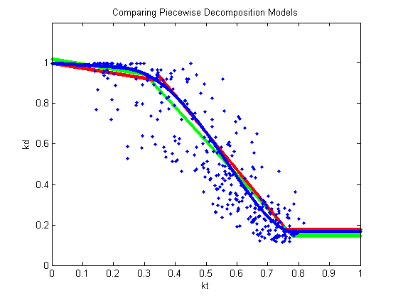
The figure below compares these three simple models and shows hourly average irradiance data collected in Florida, USA for September 2013.

Reindl et al. Decomposition Model 2
This second model form from Reindl et al., 1990 uses the same data as the first version of the model but added solar elevation ($$\Theta{_e}{_l}$$) as another variable.
$$k_d=1.02-0.254k_t+0.0123\sin\left(\theta_{el}\right):\left(k_t\leq0.3\right)$$
$$k_d=1.4-1.749k_t+0.177\sin\left((\theta_{el}\right):\left(0.3<k_t<0.78\right)$$
$$k_d=0.486k_t-0.182\sin\left(\theta_{el}\right):\left(k_t\geq0.78\right)$$
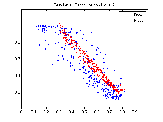
The following figure shows this model compare with the same data shown in the previous plot. Note that the addition of the solar elevation term results in more of a scatter to the data. However it is unclear if this model is actually more accurate.

