Uncertainty Quantification (UQ) involves systematically quantifying uncertainty and variability in both performance models and data. More broadly, uncertainty quantification is a component of uncertainty management – a process that involves identifying, analyzing, understanding, and mitigating uncertainties to support specific modeling or measurement goals. For solar photovoltaic (PV) performance, UQ assesses the effects of model uncertainty (which quantifies potential model error) and input variability (esp. weather) on PV performance metrics.
Why is UQ important?
The financial success of solar projects depends not only on total lifetime energy generation but also on how consistently that generation occurs and the credibility of the underlying performance model. These key aspects are driven respectively by underlying weather variability and model uncertainty. Importantly, due to the time value of energy, not every megawatt-hour generated holds equal economic value for stakeholders. Furthermore, a project’s financing takes place before the project is built; hence, stakeholders have to rely on the model accuracy of the (variable) performance predictions in typical (P50) and downside (P90 or P95 or even P99) cases. Including model uncertainty in assessing performance-variability predictions is critical to accurately assessing and mitigating financial risks associated with solar PV projects.
Project Risk Scenarios
Project performance is evaluated for both typical and downside risk scenarios for protecting the interests of various project stakeholders. UQ provides risk scenarios by a comprehensive analysis of the effects of aleatoric and epistemic uncertainties on predicted energy generation.
Typical risk scenario
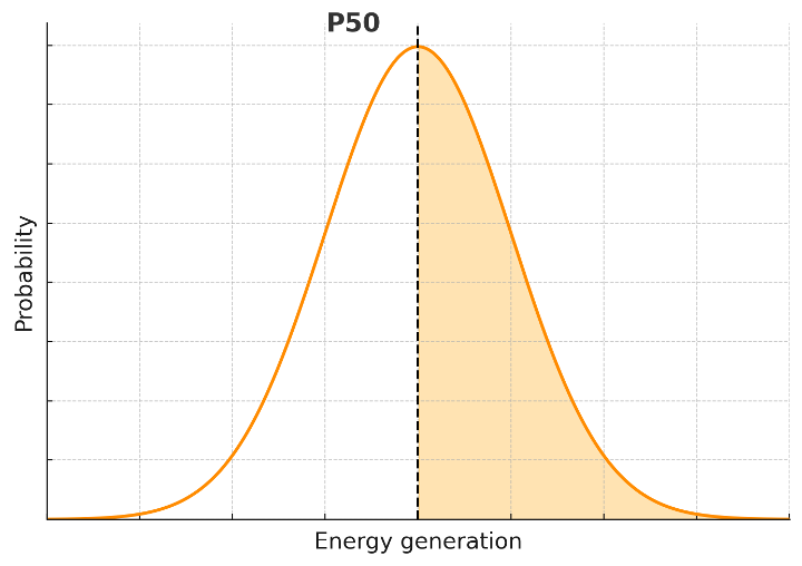
P50 is the 50th percentile (or median) of the probability distribution of predicted annual energy generation, so that 50% of the time, one should expect performance to meet or exceed the P50 value. P50 performance is considered the typical performance-risk scenario, and it is used for calculating the profitability metrics such as the internal rate of return (IRR), net present value (NPV), and multiple of invested capital (MOIC) of the project.
Downside risk scenario
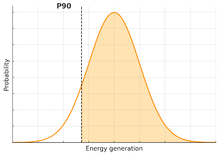
P90 is the 10th percentile of the probability distribution of predicted annual energy generation, so that 90% of the time, one should expect P90 performance or greater. P90 performance is used to guard against rarer, but also more impactful, downside performance-risk scenarios that are used in a project’s financial structuring. Most commonly, the P90 scenario is used to calculate how much debt capital the project can raise. A lower ratio of P90 to P50 (P90/P50) can indicate higher performance uncertainty (project risk), resulting in a lower fraction of debt and thus, a higher net cost of capital and lower project profitability. Depending on the specific project, a higher downside P95, or even P99, performance may be chosen to inform the financial structuring of the project. It is worth noting that highly conservative statistics such as P99 may be harder to estimate accurately due to the long tails of the underlying distribution, especially when there is sampling error or limited historical data. In such cases, the uncertainty in the uncertainty estimate itself becomes significant, and care must be taken in interpreting these extreme percentiles.
Types of Uncertainty
Uncertainties in PV performance modeling can be broadly distinguished in two types: aleatoric, or random uncertainty, and epistemic, or subjective uncertainty. Distinguishing between these types of uncertainty has benefits for the quantification of project risks.
Aleatoric Uncertainty
The aleatoric (random) uncertainty arises from inherent randomness or natural variability within the PV system or environmental factors. It cannot be reduced through additional information or measurement but is typically expected to show trends over the long term. For example, the future solar resource can be expected to have natural year-to-year fluctuations driven by weather phenomena such as El Niño which cannot be known with certainty. Some years may experience higher-than-average insolation, while others may fall below historical averages.
Epistemic Uncertainty
Epistemic (systemic) uncertainty stems from incomplete knowledge, limited data, or inaccuracies within modeling approaches. Unlike aleatoric uncertainty, epistemic uncertainty can (in concept at least) be reduced through improved measurement techniques, data collection, equipment calibration, or more sophisticated modeling. An example is the uncertainty in a module’s rated power. Uncertainty in the nominal value from a manufacturer’s datasheet can be reduced by flash testing module samples.
It’s worth noting that the distinction between aleatoric and epistemic uncertainty can depend on modeling choices and the available data. For instance, inverter outages can be treated as random events with random properties such as duration (aleatoric), modeled deterministically with an uncertain annual loss factor (epistemic), or represented as a random process (aleatoric) described by parameters with epistemic uncertainty, such as an uncertain rate of occurrence.
Advantages of Distinguishing Aleatoric and Epistemic Uncertainties
Conventionally, P50 and P90 values summarize the combined effect of both aleatoric uncertainty, due to natural resource variability, and epistemic uncertainty, which arises from model error or incomplete knowledge. Distinguishing between these two sources of uncertainty offer practical benefits.
- Quantifying Return on Investment (ROI) in Model Improvement and Data Collection: Isolating epistemic uncertainty allows stakeholders to evaluate the potential benefit of improving models, measurements, or data quality. Reducing epistemic uncertainty through such targeted investments can yield measurable improvements in the project IRR and confidence in it.
- Stakeholder-Specific Risk Profiles: For geographically diverse project portfolios, weather-related risk (aleatoric) tends to average out over the portfolio’s lifetime, reducing its overall financial impact. In contrast, model-related uncertainty (epistemic) does not benefit from such diversification and may persist consistently across assets. This presents a systemic risk, particularly for stakeholders with ownership interests or contractual obligations tied to generation thresholds, emphasizing the importance of minimizing epistemic uncertainty through improved modeling and data practices.
Asymmetrical yield forecasts
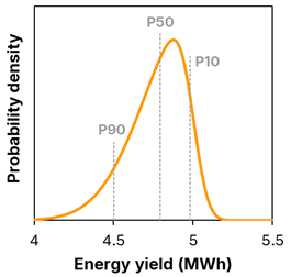
Variation in annual insolation is commonly modelled by a normal distribution for convenience. Normal distributions are symmetric about the median, or P50 of annual insolation. PV system energy yield, however, is likely to be asymmetric about the P50. A favorable year of insolation may increase yield relative to a forecast P50, but the increase is limited by factors such as AC capacity. Unlike the solar resource, system performance has no upside relative to a perfectly operating design, only downside. Outages, inverter clipping, curtailment, power factor, and degradation can all reduce annual yield below forecast, but none increase yield. At the portfolio level, this manifests as a long downside tail in yield outcomes. This negative skew can arise when reductions in yield during poor years tend to be greater than increases in yield during favourable years. Alternatively, it can arise when the losses from a poorly performing project tend to be greater than the gains from a well-performing project. The figure below presents an example of an asymmetric yield forecast, characterised by its ‘downside tail’ being broader than its ‘upside tail’.
A kWh Analytics study gives an example of a skewed distribution of availability in a portfolio [1, 2]. In an evaluation of hundreds of solar projects, both the median inverter availability and the median grid availability were ~98% (i.e. P50), but a long downside tail meant that the mean values were closer to 97% and 96%, respectively. In several projects both inverter and grid availability were less than 90%. In short, the variability in these projects was asymmetric with a strong negative skew.
Luminate gives another example of a negative skew in the yield from 29 projects [3]. After correcting for curtailment, availability and irradiance, they found that the median difference between performance and modelling was –2.7%, and that 7 projects operated at 3% below the median, whereas only 1 project operated at +3% above the median. Thus, the downside tail was much longer than the upside tail.
Understanding and accounting for sources of asymmetry is therefore critical for making realistic yield forecasts.
Sources of asymmetry
There are many possible sources of asymmetry in a yield forecast, including curtailment, availability, interannual variability in weather, soiling, clipping, and degradation.
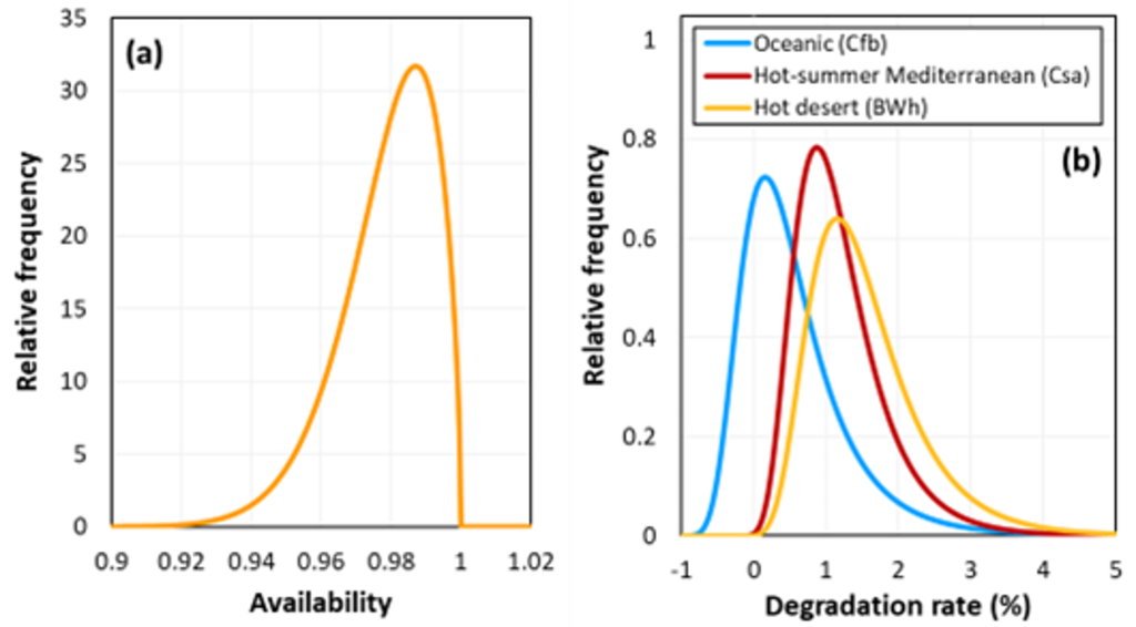
The figure below presents two examples, plotting distributions for (a) availability, as derived by Chawla from Natural Power [4] from 68 projects using 1,800 months of operational data; and (b) the annual degradation rate of silicon modules in three climates, as deduced by Tang et al. [5] from data compiled by Jordan et al. [6].
Both of these probability distributions are asymmetric and lead to negative skew in yield forecasts. (A higher degradation rate leads to a lower yield.)
Accounting for asymmetric sources of uncertainty
The practical consequence of ignoring asymmetry is a yield forecast that is systematically optimistic, not just in the downside case, but also the P50. When input distributions are treated as symmetric, energy yield forecasts tend to be overstated, and financial risk understated. Correctly characterising asymmetric uncertainty is therefore an important consideration in producing accurate and reliable yield forecasts.
There are two main approaches to combining asymmetric sources of uncertainty in a yield forecast.
The first approach fits Gaussian (normal) distributions to the downside tail of the input distributions and then combines the various Gaussian distributions via the standard root-sum-of-squares method. This approach is quick and consistent with conventional yield forecasting and preferentially captures the contribution of the downside (e.g., P95, P90, P75), which is of more interest to financiers. However, it is likely to overestimate the yield at all P-values and also cannot capture any complicated uncertainty distributions, like those with multiple peaks, or interdependencies between inputs.
The second approach is the Monte Carlo approach, which samples directly from the input distributions and numerically propagates the sampled values through the performance model to generate a distribution of outcomes. The resulting output distribution accounts for asymmetries and interdependencies in the input distributions.
References
[1] kWh Analytics, Solar Generation Index, 2022.
[2] Rasmussen H. and Browne B., “Bringing solar availability assumptions back down to earth: the case for adjusting to 97%,” PV Tech, May 2024, pp. 76–80.
[3] Luminate, “Luminate 2023 solar validation study,” white paper.
[4] Chawla D. 2024, “A database assessment of solar project availability in the United States,” white paper, Natural Power.
[5] Tang Y., Poddar S., Kay M., Rougieux F. E. Understanding and Reducing the Risk of Extreme Photovoltaic Degradation. IEEE Journal of Photovoltaics. 2025 Dec 4;16(1):150-9.
[6] Jordan D. C., Kurtz S. R., VanSant K., Newmiller J. Compendium of photovoltaic degradation rates. Progress in Photovoltaics: Research and Applications. 2016 Jul;24(7):978-89.
Content for this page was provided by Chetan Chaudhari (PowerUQ), Mark Campanelli (PowerUQ) and reviewed by Keith McIntosh (PV Lighthouse – SunSolve), Daniel Moghtader (VDE), and Cliff Hansen (Sandia National Laboratories) – 2026