This example uses May 18th, 2014 irradiance data collected at Sandia National Laboratories in Livermore, CA to demonstrate use of the wavelet variability model (WVM).
Contents
load data
This file contains two vectors: “GHI” which is the GHI measurements, and “dt” which is the timestamps.
Livermore=load('./example_data/Livermore_Sample_GHI');
Livermore_polygon=load('./example_data/Livermore_Sample_Polygon_Vertices');

% Also load the polygon vertices.
define variables
First, define the irradiance sensor variables.
irr_sensor.irr=Livermore.GHI; %measured irradiance
irr_sensor.time=Livermore.dt; %timestamps
irr_sensor.Lat=37.676208; %sensor latitude
irr_sensor.Lon=-121.703118; %sensor longitude
irr_sensor.alt=200; %sensor altitude (in meters)
irr_sensor.tilt=0; %tilt = 0 for GHI sensor
irr_sensor.azimuth=180; % 180 = due south
irr_sensor.UTCoffset=-8; %sensor UTC offset
Then define the PV plant details.
plantinfo.tilt=10; %assume modules tilted 37 degrees (approximately latitude tilt)
plantinfo.azimuth=210; %assume modules facing south
plantinfo.type='polygon'; %assume a square-shaped PV plant
plantinfo.MW=30; %assume a 30MW plant
%NOTE: we do not need to define plantinfo.PVdensity since the plant area is
%known through the polygon vertices. The calculated PV density will be
%returned to the MatLab command line: make sure it is a reasonable value!
plantinfo.Lat=Livermore_polygon.polygonlats;
plantinfo.Lon=Livermore_polygon.polygonlons;
Finally, define the cloud speed.
cloud_speed=10; %assume cloud speed of 10 m/s
run WVM
[smooth_irradiance,other_outputs]=pvl_WVM(irr_sensor,plantinfo,cloud_speed);
The PV density based on the polygon inputs was 95W/m2
plot the WVM results
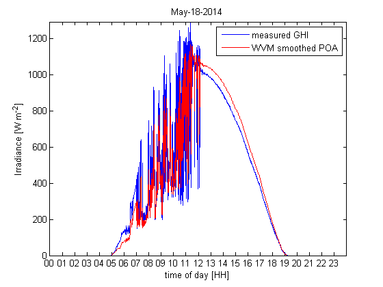
Zoomed out plot comparing the measured GHI to the WVM output of smoothed POA irradiance.
plot(irr_sensor.time,irr_sensor.irr,'b',irr_sensor.time,smooth_irradiance,'r');
legend('measured GHI','WVM smoothed POA');
set(gca,'xtick',floor(nanmean(irr_sensor.time)):1/24:ceil(nanmean(irr_sensor.time)));
datetick('x','HH','keepticks','keeplimits');
xlabel('time of day [HH]');
ylabel('Irradiance [W m^{-2}]');
axis tight
title(datestr(nanmean(irr_sensor.time),'mmm-dd-yyyy'))
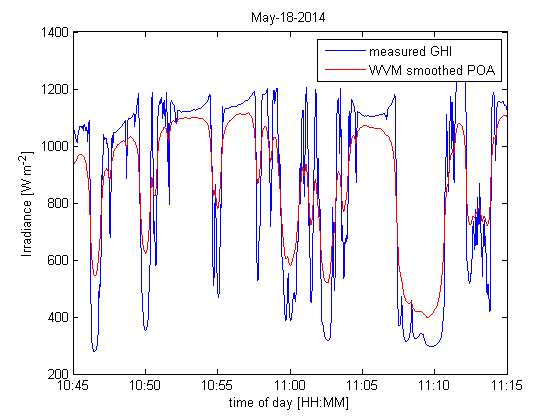
Zoomed in plot comparing the measured GHI to the WVM output of smoothed POA irradiance.
plot(irr_sensor.time,irr_sensor.irr,'b',irr_sensor.time,smooth_irradiance,'r');
legend('measured GHI','WVM smoothed POA');
set(gca,'xtick',floor(nanmean(irr_sensor.time)):1/(24*12):ceil(nanmean(irr_sensor.time)));
datetick('x','HH:MM','keepticks','keeplimits');
xlabel('time of day [HH:MM]');
ylabel('Irradiance [W m^{-2}]');
xlim([floor(nanmean(irr_sensor.time))+10.75/24 floor(nanmean(irr_sensor.time))+11.25/24])
title(datestr(nanmean(irr_sensor.time),'mmm-dd-yyyy'))